Subscribe Recommend		The 2007 retro HP 35s programmable calculator. Curve Fitting for the HP 35s Programmable Calculator Hewlett-Packard's new-for-2007 HP 35s programmable scientific calculator isn't historical yet, but it has the HP quality, look, and feel that has been missing for over a decade. The 35s is more like HP's historical offerings than it is like their other current products, which is a good thing. Since I used to enjoy programming calculators when I was younger and hadn't done so in years, I decided to tackle some largish (for a calculator) programs on my brand new HP 35s. In addition to this curve fitting program, I've written a matrix multi-tool. Both the HP-41C/CV/CX Advantage Pac and the HP-42S calculator contain a curve fitting function which can fit a sequence of (x,y) data pairs to a straight line, logarithmic, exponential, or power curve. The much newer HP 35s will only fit points to a straight line. The manual provides a program to handle the other curve types, but that program has two drawbacks: you must decide in advance which curve you want to fit to the data, and it uses up a large number of labels (the machine has only 26). The program presented below rectifies both of these issues. It uses only a single label, and it allows you to fit multiple curves to the same data set. Like the HP-41/42 programs, it also has a best-fit mode wherein it automatically chooses the curve with the best correlation coefficient. The available curves are: Linear: y = m x + b Logarithmic: y = m ln x + b Exponential: y = b em x Power: y = b xm The logarithmic and power curves require that all the x values be positive. Similarly, the exponential and power curves require that all the y values be positive. After choosing a curve to fit, or having the program choose one for you, you can predict values of y for given x values, or vice versa. Using the Program This program is integrated as closely as possible with the HP35s' built-in statistical registers and functions. Before entering a new data set, clear the statistics registers by pressing CLEAR 4Σ. Then press XEQ C ENTER to run the curve fitting program. 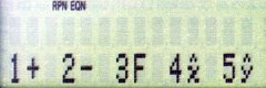This will display the main menu, which looks like this: The menu choices are: Go to data entry mode. Delete the last data pair entered. Go to the curve fitting menu. Compute x given a y value. Compute y given an x value. Pressing R/S without selecting a choice exits the curve fitting program (this is important, to ensure flag 10 is cleared so equations will work in other programs). Data Entry Mode Press 1 R/S to go to data entry mode. The X-register of the display will show the number of points entered so far (which will be zero if you had just cleared the statistics registers). To enter a data pair, first enter the y value, press ENTER, enter the x value, and press R/S. The program will briefly display RUNNING, and then display the updated number of points (the Y-register will contain the y value just entered). When you've completed data entry, press XEQ C ENTER to return to the main menu. Deleting the Last Entry If you've made a mistake entering a data pair, here's how to correct it: If you haven't pressed R/S yet, just enter the correct data pair and then press R/S. If you have pressed R/S already, press XEQ C ENTER to return to the main menu, and then press 2 R/S to select the delete data option. This will delete the last data pair entered, and return you to data entry mode (the X-register will contain the number of points entered, which will be one less than it was previously, and the Y-register will contain the y value of the point just deleted). Curve Fitting If you're still in data entry mode, press XEQ C ENTER to return to the main menu. 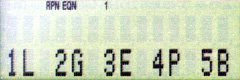Then press 3 R/S to display the curve fitting menu: The menu choices are: LINear LOGarithmic EXPonential POWer Best Fit Select the type of curve you want by pressing the corresponding number, followed by R/S. If you select best fit (5 R/S), the program will run for a few seconds to find the best fit. If you select a model that is disallowed by your data (for example, a negative y data value rules out the exponential and power curves), the program will display INVALID MODEL. Pressing R/S will take you back to the curve fitting menu for another try. Next, the curve type you or the program chose will be displayed (one of LIN, LOG, EXP, or POW). Press R/S to continue. The program will then display the value of m for the chosen curve type. For example, M= -25.94960. Press R/S to continue. Next the program will display the corresponding b value. For example, B= 84.94137. Once again, press R/S to continue. Finally the absolute value of correlation coefficient r is displayed. For example, R= 0.99973. Pressing R/S one last time will return you to the main menu. Pressing R/S without selecting a choice from the curve fitting menu will return you to the main menu. Predicting x Given y From the main menu, press 4 R/S to go to x-prediction mode. The program will prompt you with Y?. Enter a y value and press R/S. The corresponding x value will be displayed. For example, X= 23.51674. Press R/S again to be prompted for another y value, or press XEQ C ENTER to return to the main menu. Predicting y Given x From the main menu, press 5 R/S to go to y-prediction mode. The program will prompt you with X?. Enter an x value and press R/S. The corresponding y value will be displayed. For example, Y= 4.73007. Press R/S again to to be prompted for another x value, or press XEQ C ENTER to return to the main menu. Other Statistics This program uses the HP 35s' built-in statistics registers (n, Σx, etc.) to accumulate the linear coefficients, the same way the built-in statistics functions do. This means you can do the following at any time while using this program: Perform a linear fit to your data and make predictions using it via the  L.R menu. Examine the stored linear coefficient sums with the  SUMS menu. Determine the x and y means using the  x,y menu. Compute the x and y sample and population standard deviation with the  s,σ menu. Program Listing Line Instruction Comments C001←   LBL C  Display main menu C002  CLx    C003  SF 10    C004  EQN 1+ 2− 3F 4x^ 5y^  Note: x^ and y^ are from the L.R menu C005  CF 10    C006  x=0?  Decode menu choice C007  RTN    C008  1    C009  x=y?    C010  GTO C034  Go to data entry C011  R↓    C012  2    C013  x=y?    C014  GTO C029  Undo previous entry C015  R↓    C016  3    C017  x=y?    C018  GTO C101  Go to curve fit menu C019  R↓    C020  4    C021  x=y?    C022  GTO C200  Go to forecast x C023  R↓    C024  5    C025  x=y?    C026  GTO C213  Go to forecast y C027  XEQ C226  Invalid command C028  GTO C001  Return to main menu C029←   RCL Y  Recall previous entry C030  RCL X    C031  SF 0  Set removal flag C032  Σ−    C033  GTO C048  Go to data add routine C034←   n  Get number of data points C035  x≠0?    C036  GTO C046  Jump to data entry if not first point C037  STO P  Clear extended sigma registers C038  STO Q    C039  STO S    C040  STO T    C041  STO U    C042  STO V    C043  STO W    C044  CF 3  No curve type ruled out yet C045  CF 4    C046←   STOP  Stop for data input, displaying n C047  Σ+  Add data to built-in sigma registers C048←   R↓  Add data to extended sigma registers C049  STO Y    C050  x≤0?    C051  SF 4  Rule out exponential and power C052  ENTER    C053  ENTER    C054  LASTx    C055  STO X    C056  x≤0?    C057  SF 3  Rule out logarithmic and power C058  x>0?    C059  LN    C060  FS? 0    C061  +/−    C062  STO+ P  Accumulate ln(x) C063  LASTx    C064  R↑    C065  x>0?    C066  LN    C067  FS? 0    C068  +/−    C069  STO+ S  Accumulate ln(y) C070  x2    C071  FS? 0    C072  +/−    C073  STO+ T  Accumulate ln(y)2 C074  R↓    C075  LASTx    C076  ×    C077  STO+ U  Accumulate x ln(y) C078  R↓    C079  ENTER    C080  ENTER    C081  LASTx    C082  ×    C083  FS? 0    C084  +/−    C085  STO+ W  Accumulate ln(x) ln(y) C086  R↓    C087  x2    C088  FS? 0    C089  +/−    C090  STO+ Q  Accumulate ln(x)2 C091  R↓    C092  LASTx    C093  ×    C094  STO+ V  Accumulate y ln(x) C095  R↓    C096  CF 0    C097  GTO C034  Prepare to fetch next data pair C098←   SF 10  Message for ruled out models C099  EQN INVALID MODEL    C100  CF 10    C101←   CLx  Curve fitting menu C102  SF 10    C103  EQN 1L 2G 3E 4P 5B    C104  CF 10    C105  x=0?  Decode curve fitting choice C106  GTO C001  Return to main menu C107←   CF 1  Set flags for linear fit C108  CF 2    C109  1    C110  x≠y?    C111  GTO C116  User didn't select linear C112  SF 10    C113  EQN LIN    C114  CF 10    C115  GTO C193  Compute linear coefficients C116←   R↓    C117  2    C118  x≠y?    C119  GTO C127  User didn't select logarithmic C120  FS? 3  Is logaraithmic fit allowed? C121  GTO C098  Invalid model C122  SF 1  Set flags for logarithmic fit C123  SF 10    C124  EQN LOG    C125  CF 10    C126  GTO C193  Compute logarithmic coefficients C127←   R↓    C128  3    C129  x≠y?    C130  GTO C138  User didn't select exponential C131  FS? 4  Is exponential fit allowed? C132  GTO C098  Invalid model C133  SF 2  Set flags for exponential fit C134  SF 10    C135  EQN EXP    C136  CF 10    C137  GTO C193  Compute exponential coefficients C138←   R↓    C139  4    C140  x≠y?    C141  GTO C152  User didn't select power C142  FS? 3  Is power fit allowed? C143  GTO C098  Invalid model C144  FS? 4  Is power fit allowed? C145  GTO C098  Invalid model C146  SF 1  Set flags for power fit C147  SF 2    C148  SF 10    C149  EQN POW    C150  CF 10    C151  GTO C193  Compute power coefficients C152←   R↓    C153  5    C154  x=y?    C155  GTO C158  User selected best fit C156  XEQ C226  Invalid command C157  GTO C101  Return to curve fitting menu C158←   CF 1  Compute correlation for linear C159  CF 2    C160  1    C161  STO M    C162  XEQ C301    C163  SF 1  Compute correlation for logarithmic C164  FS? 3  ...but only if logarithmic allowed C165  GTO C172  Skip power, straight to exponential C166  XEQ C301    C167  x<y?  Choose the better of the two C168  GTO C171    C169  2    C170  STO M    C171←   x↔y    C172←   SF 2  Compute correlation for power C173  FS? 4  ...but only if power allowed C174  GTO C191  Exponential isn't allowed either C175  FS? 3    C176  GTO C183  Try exponential C177  XEQ C301    C178  x<y?  Choose the better of the two C179  GTO C182    C180  4    C181  STO M    C182←   x↔y    C183←   CF 1  Compute correlation for exponential C184  FS? 4  ...but only if exponential allowed C185  GTO C191    C186  XEQ C301    C187  x<y?  Choose the better of the two C188  GTO C191    C189  3    C190  STO M    C191←   RCL M  Set up for best fitting curve C192  GTO C107    C193←   XEQ C285  Compute m (slope) C194  XEQ C290  Compute b (intercept) C195  XEQ C301  Compute r (correlation coefficient) C196  VIEW M  Display m, b, and r C197  VIEW B    C198  VIEW R    C199  GTO C001  Return to main menu C200←   INPUT Y  Input y to forecast x C201  FS? 2    C202  LN    C203  RCL B    C204  FS? 2    C205  LN    C206  −    C207  RCL÷ M    C208  FS? 1    C209  ex    C210  STO X  Store and dispaly result C211  VIEW X    C212  GTO C200  Prompt for another y value C213←   INPUT X  Input x to forecast y C214  FS? 1    C215  LN    C216  RCL× M    C217  RCL B    C218  FS? 2    C219  LN    C220  +    C221  FS? 2    C222  ex    C223  STO Y  Store and display result C224  VIEW Y    C225  GTO C213  Prompt for another x value C226←   SF 10  Error for invalid menu choice C227  EQN INVALID CMD    C228  CF 10    C229  RTN    C230←   FS? 1  Recall appropriate Σ x for model C231  GTO C234    C232  Σx    C233  RTN    C234←   RCL P  Σ ln(x) C235  RTN    C236←   FS? 1  Recall appropriate Σ x2 for model C237  GTO C240    C238  Σx2    C239  RTN    C240←   RCL Q  Σ ln(x)2 C241  RTN    C242←   FS? 2  Recall appropriate Σ y for model C243  GTO C246    C244  Σy    C245  RTN    C246←   RCL S  Σ ln(y) C247  RTN    C248←   FS? 2  Recall appropriate Σ y2 for model C249  GTO C252    C250  Σy2    C251  RTN    C252←   RCL T  Σ ln(y)2 C253  RTN    C254←   FS? 1  Recall appropriate Σ xy for model C255  GTO C262    C256  FS? 2    C257  GTO C260    C258  Σxy    C259  RTN    C260←   RCL U  Σ x ln(y) C261  RTN    C262←   FS? 2    C263  GTO C266    C264  RCL V  Σ y ln(x) C265  RTN    C266←   RCL W  Σ ln(x) ln(y) C267  RTN    C268←   XEQ C230  Σ x C269  XEQ C242  Σ y C270  ×    C271  n    C272  ÷    C273  +/−    C274  XEQ C254  Σ xy C275  +    C276  RTN  Return Σ xy - Σ x Σ y / n C277←   XEQ C230  Σ x C278  x2    C279  n    C280  ÷    C281  +/−    C282  XEQ C236  Σ x2 C283  +    C284  RTN  Return Σ x2 - (Σ x)2 / n C285←   XEQ C268  Σ xy - Σ x Σ y / n C286  XEQ C277  Σ x2 - (Σ x)2 / n C287  ÷    C288  STO M    C289  RTN  Return slope (m) C290←   XEQ C230  Σ x C291  RCL× M    C292  +/−    C293  XEQ C242  Σ y C294  +    C295  n    C296  ÷    C297  FS? 2    C298  ex    C299  STO B    C300  RTN  Return intercept (b) C301←   XEQ C268  Σ xy - Σ x Σ y / n C302  x2    C303  XEQ C277  Σ x2 - (Σ x)2 / n C304  ÷    C305  XEQ C242  Σ y C306  x2    C307  n    C308  ÷    C309  +/−    C310  XEQ C248  Σ y2 C311  +    C312  ÷    C313  √x    C314  STO R    C315  RTN  Return correlation coefficient (r) Length: 1023, Checksum: EC35 Registers and Flags Register Use B Coefficient b (intercept) M Coefficient m (slope) P Σ ln(x) Q Σ ln(x)2 R Correlation coefficient r S Σ ln(y) T Σ ln(y)2 U Σ x ln(y) V Σ y ln(x) W Σ ln(x) ln(y) X Last entered or predicted x Y Last entered or predicted y Σx Σ x Σx2 Σ x2 Σy Σ y Σy2 Σ y2 Σxy Σ xy n Number of data points Flag Meaning 0 Set during removal of previous data pair 1 Logarithmic or power model selected 2 Exponential or power model selected 3 Logarithmic and power models disallowed 4 Exponential and power models disallowed 10 Set temporarily to use equations as prompts Revision History 2007-Oct-17 — Initial release. 2007-Dec-16 — Changed x-prediction and y-prediction routines to prompt for further y or x input respectively instead of returning to the main menu each time. Use XEQ C ENTER to return to the menu. I've found this to be more convenient than having to repeatedly select option 4 or 5 from the main menu when making multiple predictions. Why I Wrote this Program One of my first programmable calculators was a Texas Instruments SR-52 that I purchased at Eaton's for $149 back in 1978 or so. At that time, the TI-59 had already been introduced and the store was clearing out the SR-52. This calculator had 224 steps of program memory, 20 registers, and a magnetic card reader. It was only slightly less powerful than the HP-67. One of the programs in the very comprehensive SR-52 programming manual was a curve fitting program somewhat like the one presented here, except that it only supported linear and exponential curves, and one had to choose the curve type before entering data. What was interesting about this program was that it was presented in great detail, complete with the design processes that went into it. It was the study of TI's program and the design methods that made me really comfortable with programming their calculator. And of course, the program was useful. Now, almost 30 years later, an expanded version of this program came to mind as an ideal first project on the HP 35s, especially since my earlier HP calculators (41CX with Advantage Pac, and 42S) had this capability built in. A curve fitting tool such as this one is useful in some of my other work, such as the development of MotoCalc when I'm trying to determine a mathematical model to fit empirical data. Other HP Calculator Programs I've written programs for many of the HP calculators calculators in my collection. You may be interested in some of these: HP 35s Matrix Multi-Tool HP-41C/CV/CX Low-Sensitivity Sallen-Key Filter Design Op-Amp Gain and Offset Stage Design Op-Amp Oscillator Design HP-67 Low-Sensitivity Sallen-Key Filter Design Op-Amp Gain and Offset Stage Design Op-Amp Oscillator Design Resistor Networks of 1 or 2 Nodes     Buy Stefan a coffee! If you've found this article useful, consider leaving a donation to help support stefanv.com   Last updated Saturday December 6, 2008. E-mail Stefan   Disclaimer: Although every effort has been made to ensure accuracy and reliability, the information on this web page is presented without warranty of any kind, and Stefan Vorkoetter assumes no liability for direct or consequential damages caused by its use. It is up to you, the reader, to determine the suitability of, and assume responsibility for, the use of this information. Copyright: All materials on this web site, including the text, images, and HTML mark-up, are Copyright © 2009 by Stefan Vorkoetter unless otherwise noted. All rights reserved. Unauthorized duplication prohibited. You may link to this site or pages within it, but you may not link directly to images on this site, and you may not copy any material from this site to another web site or other publication without express written permission. You may make copies for your own personal use.